06 Apr 2017
We all know that drugs are used as treatments for diseases, right? But did you think about how, scientifically, it is shown that drugs actually benefits and but not harms? Before my biostats education, I was naively imagining that since we know what causes the disease and which part of the body it affects etc., scientist are producing chemicals to cure the diseases. But, of course, this was so naive and human body is so complicated, and mostly we don’t know even the causes of the diseases. Then, I learned that, clinical studies are conducted to show whether a drug works or not .
Let`s imagine that if anybody who developed a disease die without exception (in other words outcome of disease is invariable). Then, if we give our drug to one diseased person, and to see that he/she lives, that would be an indication for the value of drug. But we know that the outcome of disease, patients and their reaction to drugs are all vary.
So, we need to give the drug to many patients, and then analyse the results. But do we need a representative sample of the patients from whole population (for example from one country) to obtain unbiased results? Finding such people would be very hard. But still, let say we found 100 people who are representative, and give them drugs. By the way, let assume that our aim is reducing the blood pressure, so we took the number of diastolic blood pressure from 100 people before they receive the drug (baseline) and after they receive it (follow-up). So, below figure is the difference of the number of diastolic blood pressure from baseline to follow-up:
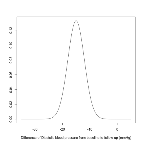
OK, results are almost all negative, that means blood pressure is decreasing (which was our aim), so we can conclude that drug works, right? Actually, no. The thing is although patients are recovered, we don’t know which of the patients who recover do so because of the drug or because they would have done so anyway. Therefore, we need another 100 patients who enter the clinical trial but do not take the drug: so-called control group (treatment group was the first one). Here, an important point is that the baseline of the treatment group and control group should be similar, otherwise the results may depend on the baseline, that mean we won`t get any reliable results.
One way to get comparable groups is that taking two representative samples from whole population, and making one group treatment group and the other control group. But this is way more costly and hard.
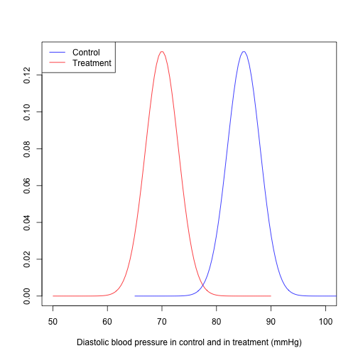
Another option is the randomization. If there are 200 patients who are eligible to enter the experiment, we randomly assign them to either control group or treatment group (randomized controlled trial (RCT)). Now we have comparable groups. Then, we see results like that
One of the coolest thing with RCTs is that we don’t need any representative sample from whole population. Let me explain why.
Below you see a diagram which explains how patients are entered to an RCT.
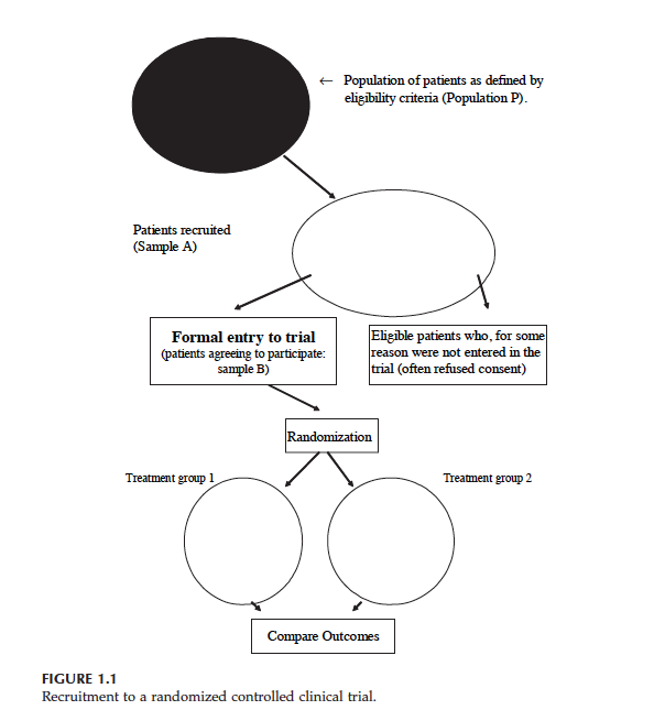
At the top you see population P. We want to know whether drug works in population P. But then, we have some patients who are eligible to trial (Sample A), lastly we have Sample B which includes the eligible patients who give their consent to enter the RCT (Treatment 1 is control group and Treatment 2 is treatment group).
Let say, the outcome measured on each individual (for example blood pressure) is a random variable . Say (if we do not give any drug to sample B) and where is true treatment effect (if we give the drug to sample B). And let say, and are mean of control group and treatment group (after randomization).
Then, and , since both control group and treatment groups are random sample from Sample B. Then, . Statistically speaking we have an unbiased estimate of treatment effect .
As you see, we did not care that sample B (or A) is a random sample from population P. Even if in population P is very different from , our estimate of is still unbiased.
Another important feature of a RCT is that by design, possible confounding factors are controlled. This is the crucial difference between observational studies and RCTs. Because of these and some other important reasons, RCTs are generally considered as gold standard. But sometimes it is just not possible to conduct an RCT. For example, you wonder if there is an association between smoking and lung cancer. So what you need is that finding people, and after randomization you need to force half of them to smoke, right? But of course this is completely unethical. So in similar scenarios, and also because RCTs are more costly than observation studies, we have to make use of observational studies. Therefore, in general, when we want to generalize our results from the sample to target population, we either need the randomization (Randomized clinical trial) or representative sample (observational studies).
Lastly, there is another source of evidence which is regarded even more reliable than an RCT, and I will try to explain it in the next post.
Note: I took the diagram and definitions from the book: “Introduction to Randomized
Controlled Clinical Trials” (Second edition) written by John N. S. Matthews.
05 Feb 2017
You may wonder what connects the plane crashes to household furniture, right? In both of those situations, there is a probability of dying attached to them. Maybe you already read stuff like 6 Things More Likely To Kill You Than A Plane Crash or this. You may see such news after a plane crash occurred in the world, and basically their take home message is that plane crashes is not that common as we might normally think. OK, this we may already know. But the author of such articles misses an important point which is very nicely explained by this Forbes article, and I will try to elaborate in this post .
Now, let’s think about the claims of such stuff more, for example the comparison of dying by a plane crash and by a household furniture (for instance falling from a bed). In this article, it is written that the odds dying from plane crash is 1 in 11 million. And than they conclude the following statement
Your bed is not your friend. Next time you have a nap remember there is a 1 in 2 million chance of dying from falling off a bed or chair!
Therefore an average person is more likely die from falling off a bed or chair compared to plane crashes. Following this logic, should we fear more from dying when we go to sleep than a plane trip? This seems awkward, right? Now let’s take a closer look to the numbers.
If we assume there are 7.5 billion people in the world, that means annually people are killed by plane crashes (according to same article above). This looks reasonable when we look at some original sources like this, and a nice figure from the same source is shown below.
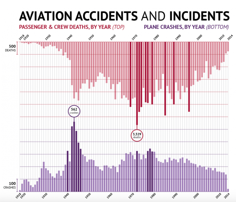
On the other hand, annually people are killed by household furniture (if we believe their numbers). Therefore, if we compare absolute risks, then household furniture are more dangerous. But what’s more relevant is actually relative risks rather than absolute risks. This is because you go to bed far more times than you use an air plane annually, right? Now let’s calculate some (very) crude relative risks to compare.
According to this source, 3.6 billion passengers were used airplanes worldwide in 2016. So 681 deaths from 3.6 billion, then relative risk is . I don’t have a source for how many times people go to bed or sit on a chair annually, but assume that any person goes 0.75 times (of course I made this number up) to bed (or chair) everyday. That means 3750 deaths from , so relative risk is . Therefore, our conclusion is that
Don’t afraid when you go to sleep even if some article says otherwise. Next time you have a nap remember the relative risk of of dying from falling off a bed or chair is 18 in 10 billion. And this is almost 105 times lower compared to dying by a plane crash.
Now, let’s think about the drowning in a bath. Our very same source says that the chance of drowning in a bath is 1 in 685,000. And if we assume that an average person use bath 0.5 times everyday (of course I don’t know any exact number). Then the relative risk is that .
OK, this may also have lower relative risk compared to plane crashes, but still maybe close right? This looks strange to me. Then I have found this WSJ article which says that in 2014, 4.866 people drowned to death in a bathtub at households in Japan. This is just too much. But they also says that 9 out of 10 involving those aged 65 or older. So this is exactly the very meaning of confounding (as I explained it in a previous post), I guess age is also an important confounding factor for dying by falling from a bed, but presumably not for dying by a plane crash. If we put it like the Turkish comedian Cem Yilmaz says, when the plane crashes, it does not matter whether your are in business class or not.
Lastly, if we look from completely different perspective, maybe all of those comparisons can be seen as redundant. Because you don’t go to bed or sit a chair as an alternative to use an airplane, right? I mean, taking bath in a bathtub is not a way of transportation, of course. And when we compare different ways of transportation, then without a doubt planes are the most safest.
08 Dec 2016
Here I want to talk about a very common mistake when it comes to life expectancy and its interpretation. In one of my epidemiology courses, the lecturer showed the below Figure.
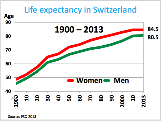
I am sure you also see graphs like that not this particular one (I mean for Switzerland) but maybe similar. OK, we see a very clear trend that life expectancy increasing in the last century. It was even doubled, right? That’s very nice. And we also see that there is clear difference between men and women but it is not my issue here.
I am more interested in the increase of the life expectancy. To understand it better first important question is, as always, why. In other words what is the possible explanation. And second question, what can we guess about the life expectancy of 2100 for example, so the prediction. My lecturer gave the answer for the first question: the remarkable achievement of modern medicine. And so by this logic, he said that the life expectancy probably may continue to increase as we had in the last century.
Now, let’s consider not 1900 but long before, for instance think about our ancestors, hunter gatherers. What we expect is that they may have similar (or even low say 30?) life expectancy like 1900, right? So lets think from a hunter gatherer perspective and see this below Figure for this purpose.

Our ancestors did not get it why they could not survive after 30. But the achievements of the medicine fully can explain it?
At this point, to understand better, we need to look at the precise definition of the life expectancy (from Wikipedia):
The mean length of life of a hypothetical cohort (all individuals born in a given year) assumed to be exposed since birth until death of all their member to the mortality rate observed at a given year.
OK, the definition seems unnecessarily complicated, but important point is that life expectancy is just a mean. So it is one type of statistical measure. But to gain more insight about the data maybe it is better to look more than just mean values. Unfortunately, I don’t have the real data, so lets just simulate some data for our purpose and plot it:
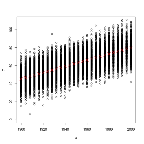
Now in the above Figure, you see all data points (the mean length of life bla bla bla per person) as well as the life expectancy as red crosses (or let’s call it mean values). But the problem is that in reality data do not look like that Figure, but instead more look like the below Figure.
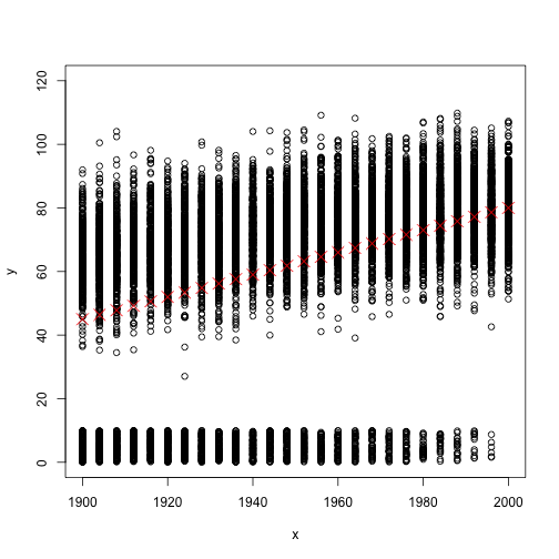
So lets compare those two Figures which are based on two different simulated datasets. Firstly the red crosses are exactly has the same values (monotonically increasing from a value close to 40 to a value close to 80). That implies mean values are the same. But in the second Figure, there are many data points very close to zero values. But the second set of data points of each given year (values which are far away to zero) seem to not increasing much. So what does that mean?. Those very small data points corresponding to children who died at very early ages (infant mortality). And as you can see, with decreasing of the infant mortality, the mean values are going away from zero even if the adult mortality stays constant.
That means, back then, your expected value of length of life is very low when you are child. But once you reach the adulthood then it is not that low like 30. That’s why even in the times when the life expectancy is 30, you can see many people of high ages like 60.
OK, I exaggerated a little bit to make the point, and of course the advancement of modern medicine (better medications etc.) is a very important explanation of the increase of life expectancy. But still I think considering only the mean values can be misleading since infant mortality has possibly more effect on the increase of life expectancy.
06 Dec 2016
There are few terms in the context of statistics which I find very interesting and powerful when I, first, understand it. One of which is, undoubtedly, the concept of confounding. This term attracted my attention; since, in my opinion, it has potential to explain many mechanisms in different fields when statistical methods are used as tools. As you may imagine, medicine, biology or political science are only some examples for different areas. To explain the confounding, I use following example.
A simple example
Now, assume that we want to examine the association between the salary per month of a person who lives in Zurich city and his or her shoe size. Of course, you may think this example is a silly one, but, I believe, by using such an example, one can understand the confounder term very easily. In order to have some data to analyse, you go to city’s most crowded street and collect data by using a questionnaire. Assume that your questionnaire is valid, you asked 1000 people (enough sample size!), so in short your data is reliable. Then you want to plot your data so as to see what is going on in the dataset. So, you decided to use a scatterplot, and you get below figure.
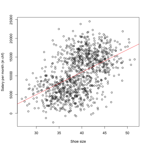
Moreover, you use simple regression, estimated the regression line and plot it as a superimposed line to the Figure (Of course I did not do any survey, I just simulated data).
Then, you concluded from this Figure as follows:
There is a strong association between shoe size and salary per month. With increasing shoe size of a person, his or her salary is increasing.
So far, everything seems you correct but still we have a weird conclusion, right? You can understand the underlying problem, when you plot the same data but now using different colors for male and female (luckily you have gender information coming from your questionnaire). And you plot two simple regression lines for female and male separately – you estimated those two lines by using two different subset of data. So we obtained the below Figure.
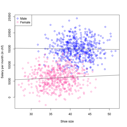
Now our conclusion is changed completely! The effect vanished, and now we don’t have any evidence suggest that there is an association between shoe size and salary. Our possible conclusion, however, is as follows. Males have substantially larger shoe size than females on average (which has a biological explanation) and also, males has earning more money on average (which is also true indeed). But shoe size has nothing to do with salary for both subset of data! In such a case, gender is a confounding variable which is mixing the effect. In this scenario, we see an effect which is not there, actually. But in other situations, you can see an effect but you may get the direction wrong.
These situations are not an extreme cases, especially if you are working with observational data. Therefore, one should try to eliminate any possible confounders. For example, if you are investigating a health-related issue, age and gender are usual suspects. But at the end of the day, it is very important not to overinterpret the results in case of any confounders.